Formulaire : Résumé Terminale S

Un résumé des notions fondamentales à connaître pour le Bac.

Complexes

$M(x,y)$ dans $(O; \vec{i},\vec{j})$ a pour affixe $z : z = x + i y$ dans $\mathbb{C}$

Le conjugué de z est : $\bar{z} = x - iy$

Module de $z : |z| = \sqrt{z\bar{z}} = \sqrt{x^2 + y^2}$

Forme trigonométrique : $z = \rho(\cos \theta + i\sin \theta)$ où $\theta = angle (\vec{i}, \overrightarrow{OM}) [2\pi]$

Forme exponentielle : $z = \rho e^{i\theta}$ (avec $|z| = \rho$ et $\theta$ = angle $(\vec{i}, \overrightarrow{OM})$ = argument de $z$)

Conjugué de $z$ : $\bar{z} = \rho e^{-i\theta}$

Soient $A$ et $B$ d'affixes $z_A$ $z_B$ alors $\overrightarrow{AB}$ a pour affixe $z_B - z_A$ et $AB = |z_B - z_A|$

Propriétés des modules

$|\bar{z}| = |z|$ ; $\bigg|\dfrac{1}{z}\bigg| = \dfrac{1}{|z|}$ ; $|zz'| = |z||z'|$

Propriétés des arguments

$\arg{zz'}= \arg z + \arg z' [2\pi]$

$\arg \bigg(\dfrac{z}{z'}\bigg) = \arg z - \arg z' [2\pi]$

Transformations usuelles

Soit une transformation telle que $M(z) \rightarrow M'(z')$

• Translation de vecteur $\vec{u}$ d'affixe $t : z' = z + t$

• Homothétie de centre $\Omega$ d'affixe $\omega$ et de rapport $k : z' - \omega = k (z- \omega)$

• Rotation de centre $\Omega$ d'affixe $\omega$ et d'angle $\theta : z' - \omega = e^{i\theta} (z- \omega)$

Equations du second degré dans $\mathbb{C}$

Soit l'équation $az^2 + bz + c = 0$ et le discriminant $\Delta = b^2 - 4ac$

• si $\Delta > 0$ alors 2 solutions réelles :

$z_1 =\dfrac{-b +\sqrt{\Delta}}{2a}$ ; $z_2 = \dfrac{-b -\sqrt{\Delta}}{2a}$

et $z_1z_2 = \dfrac{c}{a}$; $z_1 + z_2 =\dfrac{-b}{a}$

• si $\Delta = 0$ alors 1 solution réelle : $z_0 = \dfrac{-b}{2a}$

• si $\Delta < 0$ alors 2 solutions complexes :

$z_1 =\dfrac{-b + i\sqrt{\Delta}}{2a}$; $z_2 = \dfrac{-b - i\sqrt{\Delta}}{2a}$

et $z_1z_2 = \dfrac{c}{a}$; $z_1 + z_2 = \dfrac{-b}{a}$

• si $\Delta \neq 0$ alors $az^2 + bz + c = a(z - z_1) (z - z_2)$ et si $\Delta = 0$ alors : $az^2 + bz + c = a(z - z_0 )^2$

Identités remarquables

$(a + b)^3 = a^3 + 3a^2b + 3 ab^2 + b^3$

$a^3 + b^3 = (a + b) (a^2 - ab + b^2 )$

$(a - b)^3 = a^3 - 3a^2b + 3 ab^2 - b^3$

$a^3 - b^3 = (a - b) (a^2 + ab + b^2 )$

$(a + b)^n = a^n + \begin{pmatrix} n \\ 1 \end{pmatrix} a^{n-1}b+ ... + \begin{pmatrix} n \\ k \end{pmatrix} a^{n-k}b^k + .... + \begin{pmatrix} n \\ n-1 \end{pmatrix} ab^{n-1}+b^n$

Les suites

• Suites arithmétiques de raison $r$ et premier terme $u_0$ Alors : $u_{n +1} = u_n + r$ ou $u_n = u_0 + nr$

• Somme de $n$ termes consécutifs de la suite $=$ "nbre de termes" • $\dfrac{"1^{er}terme" + "dernier"}{2}$

En particulier : $1+ 2 + 3+ .........+ n = \dfrac {n(n +1)}{2}$

• Suites géométriques de raison $q$ et premier terme $u_0$ alors $u_{n +1} = q.u_n$ ou $u_n = u_0q^n$

Somme de $n$ termes consécutifs de la suite = $"1^{er} terme"$ •
$\dfrac{1- q^{nombre de termes}}{1- q}$ avec $q \neq 1$

En particulier : $1+ x + x^2 + x^3 + .........+ x^n = \dfrac{1- x^{n +1}}{1 - x}$ $(x \neq 1)$

Les fonctions logarithme et exponentielles

$e^0 =1$ ; $e^{a +b} = e^ae^b$ ; $e^{a-b} = \dfrac{e^a}{e^b}$ ; $(e^a )^b = e^{ab}$ ; $\ln{e} =1$ ;

$\ln{1}= 0$ ; $\ln{ab} = \ln {a} + \ln{b}$ ;$\ln{\dfrac{a}{b}}= ln{a} - ln{b}$

$a^x = e^{x \ln{a}}$ ; $\ln{a^x} = x \ln{a}$ ; $y= e^x \Longleftrightarrow x = \ln{y}$

Les limites usuelles de fonctions

$\lim\limits_{x \rightarrow +\infty} \ln{x}$ $= +\infty$

$\lim\limits_{x \rightarrow +\infty} e^x$ $= +\infty$

$\lim\limits_{x \rightarrow -\infty} e^x$ $= 0$

$\lim\limits_{x \rightarrow +\infty} \dfrac{e^x}{x}$ $= +\infty$

$\lim\limits_{x \rightarrow -\infty} xe^x$ $= 0$

$\lim\limits_{x \rightarrow +\infty} \dfrac{\ln{x}}{x}$ $= 0$

$\lim\limits_{x \rightarrow +\infty} \dfrac{e^x}{x^n}$ $= +\infty$

$\lim\limits_{x \rightarrow +\infty} \dfrac{\ln{x}}{x^n}$ $= 0$

$\lim\limits_{x \rightarrow -\infty} x^ne^x$ $= 0$

$\lim\limits_{x \rightarrow +\infty} x^ne^{-x}$ $= 0$

$\lim\limits_{x \rightarrow 0} \ln{x}$ $= -\infty$

$\lim\limits_{x \rightarrow 0} x\ln{x}$ $= 0$

$\lim\limits_{x \rightarrow 0} \dfrac{\sin{x}}{x}$ $= 1$

$\lim\limits_{x \rightarrow 0} \dfrac{1-\cos{x}}{x}$ $= 0$

$\lim\limits_{x \rightarrow 0} \dfrac{\ln{1+ x}}{x}$ $= 1$

$\lim\limits_{x \rightarrow 0} \dfrac{e^x -1}{x}$ $= 1$

Les dérivées primitives

Opérations et application des dérivées

• Equation de la tangente à la courbe $Cf$ en $A(a; f (a)) : y = f '(a) (x - a) + f (a)$

Calcul intégral - Les équations différentielles

Si $F$ primitive ce $f$ alors :

$\int_{a}^{b} f(t)dt = F(b)-F(a)$ et si $g(x)=\int_{a}^{x} f(t)dt$ alors $g'(x)=f(x)$

$\int_{a}^{b} f(t)dt = -\int_{b}^{a} f(t)dt$

$\int_{a}^{c} f(t)dt = \int_{a}^{b} f(t)dt + \int_{b}^{c} f(t)dt$

$\int_{a}^{b} f(t)dt = \alpha \int_{a}^{b} f(t)dt + \beta\int_{b}^{a} g(t)dt$

si $a \leqslant b$ et $f \geqslant 0$ alors

$\int_{a}^{b} f(t)dt \geqslant 0$ ; si $a \leqslant b$ et $f \leqslant g$ alors $a \int_{a}^{b} f(t)dt \leqslant \int_{a}^{b} g(t)dt$

si $a \leqslant b$ et $m \leqslant f \leqslant M$ alors $m(b - a) \leqslant \int_{a}^{b} f(t)dt \leqslant M(b-a)$

Intégration par parties

$\int_{a}^{b} u(t)v'(t) d_t= \bigg[u(t)v(t)\bigg]_{a}^{b} - \int_{a}^{b} u'(t)v(t) d_t$

Equations différentielles

Les solutions de $y'= ay + b$ sont des fonctions $f (x) = Ce^{ax} - \dfrac{b}{a}$ où $C$ est un réel.

Les Probabilités

Dénombrements

$n! = 1 \times 2 \times 3 \times … \times n$ avec $0! = 1$ et $(n+1)! = n! \times (n+1)$.

Le nombre de combinaisons de $p$ éléments pris parmi $n$ est noté $\begin{pmatrix} n \\ p \end{pmatrix}$

$\begin{pmatrix} n \\ p \end{pmatrix} = \dfrac{n(n-1)...(n-p+1)}{p!} = \dfrac{n!}{p!(n-p)!}$ ; $\begin{pmatrix} n \\ p \end{pmatrix} = \begin{pmatrix} n \\ n-p \end{pmatrix}$ ; $\begin{pmatrix} n \\ p \end{pmatrix} = \begin{pmatrix} n-1 \\ n-p \end{pmatrix} + \begin{pmatrix} n-1 \\ p \end{pmatrix}$ ; $\begin{pmatrix} n \\ 1 \end{pmatrix} = n$

Développement

$(a+b)^n = a^n + \begin{pmatrix} n \\ 1 \end{pmatrix}a^{n-1}b+...+ \begin{pmatrix} n \\ k \end{pmatrix}a^{n-k}b^{k}+...+b^n$

Généralités :

$P(A \cup B) = P(A) + P(B) - P(A \cap B)$ ; $P(\bar{A}) =1- P(A)$ ; $P(\Omega) =1$ ; $P( \oslash) = 0$

En cas d'équiprobabilité :
$P(A) = \dfrac{nombre d'éléments de A}{nombre d'éléments de \Omega}$ = $\dfrac{"nombre de cas favorables"}{"nombre de cas possibles"}$

Proba de $B$ sachant $A$ :$P_A (B) = \dfrac{P(A \cap B)}{P(A)}$; si $A$ et $B$ sont indépendants $P(A \cap B) = P(A) \times P(B)$

Trigonométrie - Produit scalaire

Formules d'addition

• $\cos{(a+b)} = \cos {a} \cos{b} - \sin{a} \sin{b}$

• $\cos{(a-b)} = \cos{a} \cos{b} + \sin{a} \sin{b}$

• $\sin {(a+b)} = \sin{a} \cos{b} + \cos{a} \sin{b}$

• $\sin{(a-b)} = \sin{a} \cos{b} - \cos{a} \sin{b}$

Formules de duplication

$\cos(2a) = \cos^2{a} - \sin^2{a} = 2\cos^2{a}-1 = 1 - 2\sin^2 {a}$

$\sin{(2a)} = 2\sin{a}\cos{a}$

Valeurs remarquables

Produit scalaire

$\vec{u}$ et $\vec{v}$ tels que $\vec{u} = \overrightarrow{OA}$ ; $\vec{v} = \overrightarrow{OB}$ ; soit $\theta = angle (\overrightarrow{OA},\overrightarrow{OB})$ alors
$\vec{u} \bullet \vec{v} = \overrightarrow{OA} \bullet \overrightarrow{OB} = OA \times OB \times cos \theta$

si $\vec{u}(x;y)$ et $\vec{v}(x';y')$ alors $\vec{u} \bullet \vec{v} = xx'+yy'$

si $\overrightarrow{OB}$ se projette en $\overrightarrow{OH}$ sur $\overrightarrow{OA}$ alors

• $\vec{u} \bullet \vec{v} = OA \times OH$ (si les vecteurs sont de même sens)
• $\vec{u} \bullet \vec{v} = -OA \times OH$ (si sens contraires)

$\vec{u}$ et $\vec{v}$ sont orthogonaux $\vec{u} \bullet \vec{v} = 0$

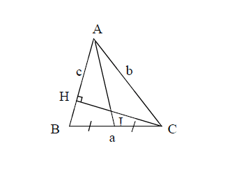
Al Khashi :

$a^2 = b^2 + c^2 - 2bc \cos{\widehat{A}}$

Théorème de la médiane :

$c^2 + b^2 = 2AI^2 + \dfrac{a^2}{2}$

Aire du triangle :

$S =\dfrac{1}{2}bc \sin{\widehat{A}}$

Formule des sinus :

$\dfrac{a}{\sin{\widehat{A}}}=\dfrac{b}{\sin{\widehat{B}}}=\dfrac{c}{\sin{\widehat{C}}}$

Equation de droite :

$ax + by + c = 0$ équation de $D$ qui admet pour vecteur directeur $\vec{u} (-b;a)$ et normal ("$\perp$") $\vec{v} (a;b)$.

Toutes nos vidéos sur les notions à connaître absolument pour le bac s